
Most CQE candidates stop at P(d = c) when the stem asks for Pa, or read the producer’s risk off the curve as if it were the probability of acceptance. Both errors are one line of thinking away from the right answer.
What does an OC curve actually show?
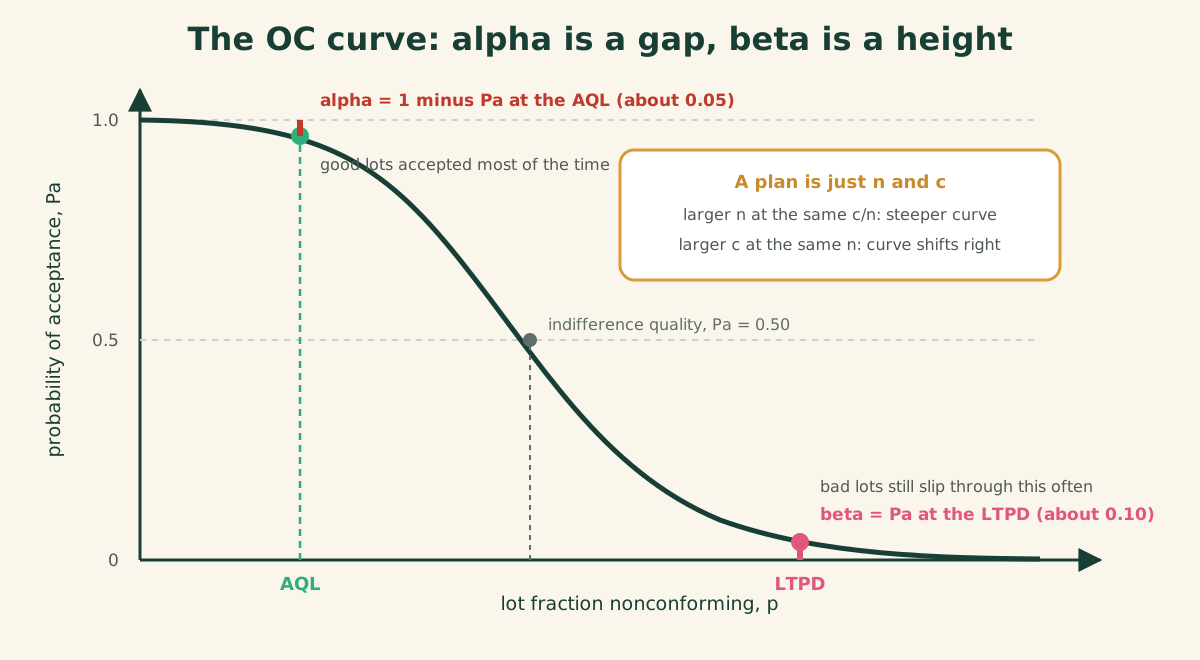
A single sampling plan by attributes is two numbers. Draw n items at random from the lot, count the nonconforming ones, d, and accept if d is at most c. The probability of acceptance, Pa, is the probability that d is at most c when the lot fraction nonconforming is p, and for a lot at least ten times the sample d is close to binomial. Plot Pa against p and you have the operating characteristic curve: 1 at p = 0, falling toward 0 as p grows.
The curve is the honest statement of what the plan does. The ideal plan would be a step, accepting everything better than some quality and rejecting everything worse. Real plans are S-shaped, and the risk lives in the S. A larger n at the same c over n ratio makes the curve steeper; a larger c at the same n shifts it right and makes the plan more forgiving.
Two things follow that surprise people. A c = 0 plan is not automatically tighter: it rejects good lots often while its tail still lets some bad lots through. And percent sampling gives protection that changes with lot size, because protection comes from n and c, not from the fraction inspected.
What are the AQL, the LTPD, alpha and beta?
Two named points on the curve define the risks. The acceptable quality level, AQL, is the worst lot quality the producer wants accepted most of the time, and the producer’s risk, alpha, is 1 minus Pa at the AQL, usually designed to be about 0.05. The lot tolerance percent defective, LTPD, also called the RQL or LQ, is the lot quality the consumer wants rejected most of the time, and the consumer’s risk, beta, is Pa at the LTPD, usually about 0.10. The indifference quality level is the p at which Pa is 0.50.
Read the definitions once more, slowly. Alpha is one minus a Pa; beta is a Pa. That asymmetry is the trap, and AQL does not mean “the quality we accept.” It is the level the plan accepts with high probability.
Worked example: Pa from the binomial for n = 50, c = 2
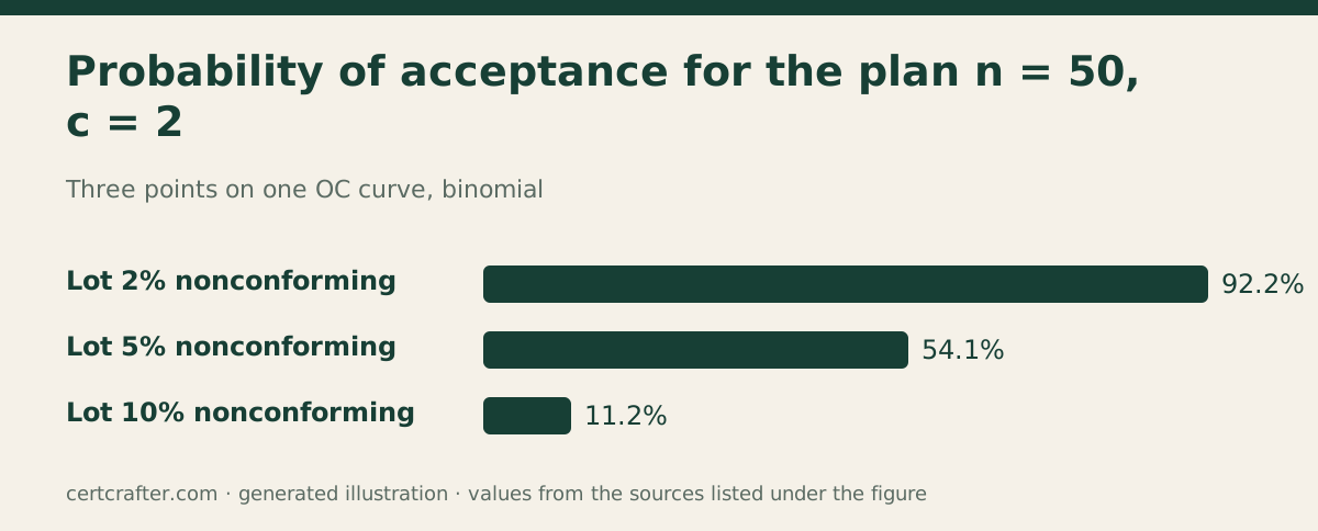
A lot of 3,000 connectors is inspected with n = 50, c = 2. Find Pa when the lot is 2% nonconforming, so p = 0.02, and accept if d is 0, 1 or 2.
- P(0) = 0.98^50 = 0.3642.
- P(1) = 50 × 0.02 × 0.98^49 = 0.3716.
- P(2) = 1225 × 0.02^2 × 0.98^48 = 0.1858, where 1225 is C(50, 2).
- Pa = 0.3642 + 0.3716 + 0.1858 = 0.9216.
A 2% lot gets through 92 times in 100. Run the same three terms at p = 0.05 and Pa is 0.5405, a coin flip; at p = 0.10 it is 0.1117, about 11 times in 100. Those are three points on one OC curve, and they say something uncomfortable: if the buyer’s LTPD is 5%, this plan leaves beta at 0.54, far above the conventional 0.10.
The plan n = 80, c = 2 against an AQL of 1% and an LTPD of 8% comes out differently: Pa at the AQL is 0.9534, so alpha is 0.0466, and Pa at the LTPD is 0.0404, so beta is 0.0404. Both sit under the conventional 5% and 10%, and both parties can sign.
The ASQ CQE Complete Exam Kit drills the Poisson shortcut, the hypergeometric case and the Z1.4 mechanics with an explanation for every option.
When does the Poisson replace the binomial?
When n is at least 20 and p at most 0.05, or np under about 5, the Poisson with its mean at np is close enough and much faster, because each term is the previous one times the mean over x. For n = 125, c = 3 at p = 0.01 it gives 0.9617 against the binomial’s 0.9626, and even at np = 5.0 the two are within 0.006. When the sample is more than about 10% of the lot, neither applies and the hypergeometric is the exact answer.
What do AOQ, AOQL and ATI mean?
When a rejected lot is 100% inspected and every nonconforming unit found is replaced, the scheme is rectifying inspection, and the quality leaving the station is better than the quality arriving. The average outgoing quality is AOQ = p * Pa * (N - n) / N, where N is the lot size: an accepted lot goes out with its N minus n uninspected units still at quality p, and a rejected lot goes out clean. When N is much larger than n, AOQ is about p times Pa.
AOQ is small when p is small, because there is little to find, and small when p is large, because most lots are rejected and screened. In between it peaks at the AOQL, the worst long-run average quality the scheme lets through. For lots of 2,000 inspected with n = 80, c = 2, AOQ at p = 0.02 is 0.02 × 0.7844 × 0.96, which is 1.51%, and the peak is 1.64% at an incoming quality near 2.81%. However bad the supplier gets, outgoing quality stays at or below 1.64%, at the price of inspecting most of each lot when p is high.
The average total inspection, ATI = n + (1 - Pa) * (N - n), is the number for budgeting labor. Every lot costs n; a rejected lot costs the remaining N minus n as well, so ATI rises from n toward N as p grows, 493.9 units per lot in that same case at p = 0.02.
How is sampling used on a real receiving dock?
In practice nobody computes Pa at the dock. The quality engineer picks an AQL per class of nonconformity, lower for majors than for minors, and the ANSI/ASQ Z1.4 tables supply a plan whose OC curve passes near Pa = 0.95 at that AQL. Lot size and inspection level give a sample size code letter; the letter and the AQL give n, the acceptance number and the rejection number for the current severity. Switching rules then move the severity with the supplier’s record: tightened is fast and automatic, reduced is slow and needs approval.
The engineer’s real job is the sample itself. Drawn at random from the whole lot, not off the top of the pallet, with the units kept traceable and the count honest. Sampling sorts lots; it does not improve them. Only rectifying inspection changes outgoing quality, and only on average.
How does the CQE exam frame sampling questions?
Numeric stems give n, c and p and ask for Pa; give the AQL and LTPD and ask for alpha or beta; or give N, n and Pa and ask for AOQ or ATI. The distractors are P(d = c) alone, alpha quoted as 0.95, AOQ without the (N minus n) over N factor, and ATI as n plus (1 minus Pa) times N. Concept stems ask what the OC curve shows, what the AOQL means, why c = 0 is not automatically better, and why percent sampling fails.
The arithmetic takes a scientific calculator two minutes. The marks are lost on the definitions.
What to do next
Work the three Pa terms above on your own calculator until the keystrokes are automatic, then try the free 20-question sample and see whether the sampling items feel the same. Unofficial: CertCrafter is not affiliated with ASQ, and ASQ does not endorse this page.
Comments
Comments are read by a person before they appear. How we moderate.